MUR Blog - LiDAR Correction

In this post, the steps taken during our LiDAR experimentation are detailed.

For testing an Ouster OS1-64 was utilized. This LiDAR is capable of polling at a rate of 10/20Hz depending on the azimuth resolution. A standard spinning LiDAR works similarly to a rolling shutter camera, in which a slice of the full image/scan is sampled at once.

This is all fine and well until the LiDAR starts moving. Which is the case of our application moving at speed (similar to a rolling shutter aliasing in cameras). With some quick napkin, a vehicle traveling at 80kph would incur a 1m deviation between the start and end of a LiDAR scanning at 20Hz. Which in our application makes the LiDAR completely useless, as the width of the track at FSAE is only 3m wide.

This deviation from the start and end of the LiDAR scan is further exacerbated when the vehicle also has an angular velocity. Which could occur during a normal track drive and guaranteed to occur during the skid-pad event (Time to complete a circle).

Thus, these errors have to be corrected before the LiDAR data can even be used for mapping. Which leads us to two options, the first is to swap the LiDAR to a solid-state LiDAR (which is akin to a global shutter camera) such that there is little to no time difference between the first and last sample of a frame. The second option is to integrate pose estimation of the vehicle and accept that we cannot poll a perfect circle but rather curve ellipse around the trajectory of the vehicle. As solid-state LiDARs are still quite experimental and pricey, we decided to move forward with option 2, integrating pose estimation for LiDAR correction.

In the naive implementation (Single poll at the start of scan) of LiDAR polling, in which the position is assumed to be the start of each 360° scan, the pose is updated at a rate of the LiDAR (10/20Hz). However, if the pose was interpolated through the LiDAR scan, we would be able to recreate/anti-alias the resultant scan into something more representative.

The use of the OS1-64, however, has a trick to make said corrections easier. The OS1-64 LiDAR outputs the LiDAR scans in bins of 16 vertical slices, such that when working with 1024 angular bins at 20Hz would give an update rate of 320Hz. Which is 3x higher than the polling rate of the internal IMU (100Hz) used for testing.

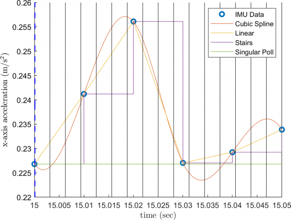
Which allows us to perform the naive IMU polling at the rate which the IMU provides data (“Stair” polling/Euler Integration), or 22cm between the 48 vertical slices (3 packets of 16 vertical slices).

Assuming the maximum speed of the vehicle is 80kph, which is 22.22m/s, and the IMU update frequency is at 100hz, this translates to about 22cm per IMU update.

The next step in refinement is the use of the trapezoidal rule for numerical integration with IMU sample points as the points of integration, which nets us a linear interpolation of vehicle pose. An even further refine step could be the use of cubic b-spline interpolation which “may” be more representative of the vehicle dynamics. However, when trying to numerically integrate the cubic spline a sparse time step will degenerate the cubic curve into a linear interpolation. Thus, it was decided for the interim to stick with a linear integration model, as higher-ordered interpolation techniques may be “pulling data out of thin air” (Making the IMU data sample rate seem higher than it is).

A quick frequency analysis of MUR’s 2017 combustion car’s IMU reading (10Hz) during its track drive (endurance), does seem to show that the characteristic/energetic vehicle dynamics at least on the acceleration scale is around 0.1 to 1Hz.

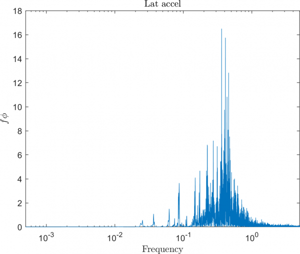
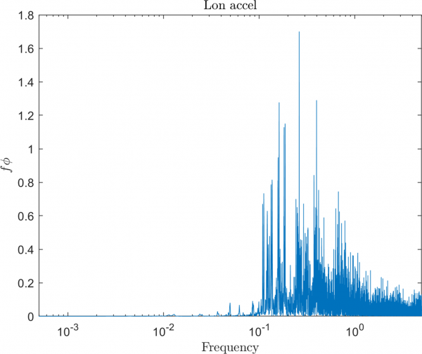
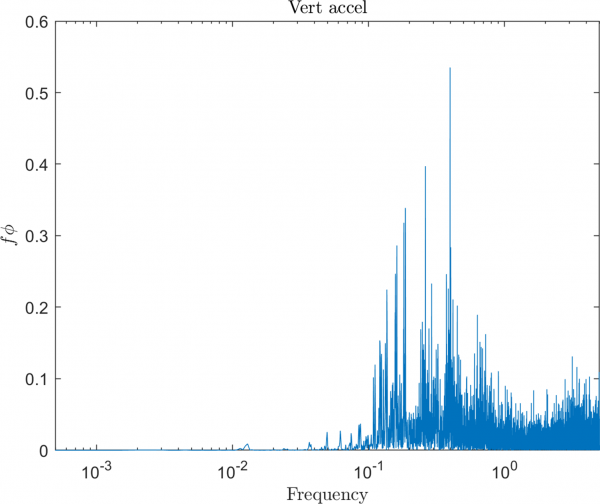
These make the initial guess of using a linear integration technique for LiDAR correction show promise, as a polling rate of an IMU at 100 Hz is 100 to 1000x greater than the characteristic vehicle dynamics, which can aid in IMU selection.

Lastly, the idea of modularity and coupling of the code architecture should be brought up. The team is still in discussion on the placement and implementation of the LiDAR correction code, as a LiDAR pipeline should not be required to do complex pose estimations. Further, in literature, various mapping algorithms have been developed to perform further sensor fusion for LiDAR correction, such as V-LOAM.

About the Author:

Andrew Huang
Spatial & Perception Engineer, 2020