MUR Blog - LiDAR Simulation, Classification and Mounting

The original plan was to head into the laboratory to work on the Husky robot at this time. However, due to these unforeseen circumstances, we ended up having to shift our main focus to simulation within Gazebo.

Optimistically, we would be able to get a few weeks of hands-on time with the Husky robot after the Stage 4 restriction ended, but it will still be a challenge to get everything running and collect all the validation data required for the final report.

LiDAR Pipeline Simulation

To ensure that the existing LiDAR pipeline can integrate smoothly with the SLAM module, a simple simulation is created for testing and integration.

TortoiseBot Robot in Gazebo Simulator

This simulation is created with reference to Wil Selby’s blog post which details the high-level steps he took to get OS1-64 LiDAR mounted on an RC car in Gazebo simulator.

By default, the Gazebo simulator uses CPU for LiDAR laser ray simulation, but this is not computationally efficient at all and scales rather badly when simulating high-resolution LiDAR such as the Ouster OS1-64. Fortunately, there exists a GPU ray plugin that allows users to simulate the LiDAR sensor with GPU. This significantly improves simulation performance and allows the CPU to focus on processing the main LiDAR pipeline.

LiDAR Cone Classification

While the previous LiDAR pipeline was able to detect traffic cones, it still lacked the capability of differentiating between the blue and yellow traffic cones, which are vital information for the path planner. The blue and yellow traffic cones define the left and right boundaries of the race track respectively.

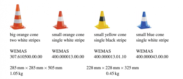
Traffic Cones specified in FSG Competition

From the image above, we can see that the traffic cones have distinct visual appearance and patterns. Specifically, the yellow cone follows a bright-dark-bright pattern, while the blue cone follows a dark-bright-dark pattern. Therefore, even without full 3-channel colour information, we may be able to differentiate between these cone types.

Approaches Considered

Initially, various approaches were considered for the LiDAR cone classification pipeline. The main options consisted of the following:

1. Use a neural network (such as PVCNN) to perform both classification and detection.
2. Build on top of the existing LiDAR pipeline by leveraging other point attributes returned by the OS1 LiDAR.

While option 1 is considered to be more robust, we currently have a limited understanding of point cloud-based neural networks, and we also lack the dataset which is required for training and testing.

Therefore, we decided to pursue option 2, which does not require a significant re-write of the existing pipeline, nor a well-constructed dataset which would be time-consuming to develop. This approach uses intensity image generated by the LiDAR to perform classification. The Ouster LiDAR also provides an img_node which provides a sample of how a developer can generate an image based on various returned attributes such as intensity, reflectivity, and ambient noise.

Point Cloud Cluster to Bounding Box

Next, we need to find a way to translate the detected traffic cone point cloud to a bounding box on the intensity image. This was achieved by performing a spherical project of all the points in the point cloud cluster, which can then be further processed to obtain an approximate bounding box on the traffic cone.

Traffic Cone Detections on Intensity Image

Data Collection & Classifier Design

A simple convolutional neural network consisting of convolutional layers and max-pool layers was trained to classify traffic cone intensity image crop-outs. The intensity image crops data were generated by cropping the approximate region of interest and resized to 32 x 32.

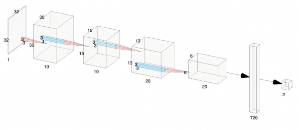
Basic CNN Design for LiDAR Image Classifier (Presented in AlexNet Style)

However, due to the limitation of working indoor, only a very limited set of training data was collected. Extensive input data augmentation along with network dropouts was applied, but the network still appeared to have overfitted, which was hinted at by the unusually high validation accuracy.

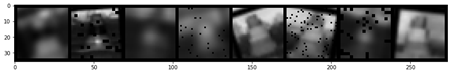
Training data after applying data augmentation

Before deployment, the classifier model and weights were saved and converted to an ONNX model, which is then optimised for Nvidia’s TensorRT framework. This allows the network to perform classification inference within 1ms with a maximum batch size of up to 50.

Classifier Performance

A mini-demo of the LiDAR detection and classification pipeline shown below. While the pipeline functions as expected, the classifier performance can definitely be improved further with future addition to the tiny classification dataset that we have at the moment.

LiDAR Classification Mini-demo (intensity image on top, point cloud at the bottom)

During indoor testing, the pipeline was able to complete one iteration of processing within 50ms. However, a stream of larger test data would be required to fully assess the maximum throughout.

A major limitation of this classifier is the vertical resolution of the LiDAR. Running in 1024 x 64 MODE, the LiDAR essentially provides access to a grey-scale image of size 1024 x 64, but when cones are further away, the cropped area significantly reduces. Assuming we need at least 6 vertical pixels on the intensity image to perform classification on the small traffic cone as specified by FSG, this limits the classification range to about 11.9m.

LiDAR Mounting Position

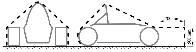
Allowed Space for Mounting Sensors (FSG 2020 Rules: DV 4.2.1)

Currently, there are two main proposals for where the LiDAR should be mounted on the MUR-20E (the 2020 electric car).

1. Mount the LiDAR below the front nose cone.
2. Mount the LiDAR above the driver headrest.

Originally, we were leaning towards option 2 for LiDAR mounting as resolves the issue of potential occlusion while trying to detect traffic cones that are directly behind another cone. However, due to the design constraints imposed by the main team, it would be significantly more challenging to mount the sensor near the headrest as that is also where the stereo camera enclosure is placed.

In the end, we settled on option 1 which should maximise the detection range but is susceptible to the problem of occlusion. This problem should not be severe as FSG rules indicate that cones are usually placed metres apart, except in sharp corners where cones would aggregate in proximity.

Future Tasks

The next step to improve the existing pipeline would be to refactor existing codes and collect an additional classifier dataset. The data collection task would most likely take place immediately after we are cleared to work on campus.

Another good outcome from the current implementation is the ability to label point cloud data. That is, given a track drive dataset, the algorithm can help label exactly which points of the point cloud belong to traffic cones of a particular type/colour. This could be useful if we transition into a supervised learning-based pipeline that required labeled point cloud dataset.

About the Author:

Steven Lee
Spatial & Perception Engineer, 2020