MUR Blog - Object Detection and Inference Optimisation

In this post, we would like to discuss the various improvements we have made to our object detection pipeline. This includes our newly improved dataset and using a newer object detection model.

Improving Upon MIT Driverless Dataset

Thanks to the open source MIT Driverless repository, other teams can start developing their object detection networks without spending a significant amount of time building and labelling their dataset. However, the MIT dataset does not include labels for the different classes of cones. That is, blue, orange, yellow. Therefore, we decided to improve upon this open-source dataset by developing a custom MATLAB GUI program to assign these class labels.

I would like to thank all the contributors who made this new dataset possible, especially Andrew Huang for developing the custom MATLAB program for this task.

Overall, we went through 7955 images and looked through:

• 24681 blue bounding boxes
• 14547 orange bounding boxes
• 45707 yellow bounding boxes
• 103 false-positive cases identified

We do not expect the new dataset to be perfect, but the object detection network should be capable of handling a small amount of mislabelled data.

YOLOv4 for Object Detection

In the previous object detection blog post, we were still using the older YOLOv3 model for cone detection.

On 23 April 2020, YOLOv4 paper was released by Alexey Bochkovskiy which establishes itself as the new state-of-the-art in terms of object detection. However, this author different to the person who developed the first 3 versions of the YOLO detection neural network. The original YOLO researcher, Joseph Redmon, made the decision to quit computer vision research citing negative societal impacts, including its use in mass-surveillance and military applications.

YOLOv4 Overview

YOLOv4 makes use of various components including Bag of Freebies and Bag of Specials.

• Bag of Freebies are methods that only change the training strategy or only increase the training cost. Common examples are data augmentations.
• Bag of Specials are plugin modules for enhancing certain attributes of a model. This includes enlarging the receptive field and improving feature integration.

One rather interesting data augmentation used in YOLOv4 was Self-Adversarial Training. During training, for every second iteration, the network performs an adversarial attack on itself.

1. Modify the training image to make the network think that there is no relevant object in the image.
2. Train the network on the modified image which should improve where the network pays attention to.

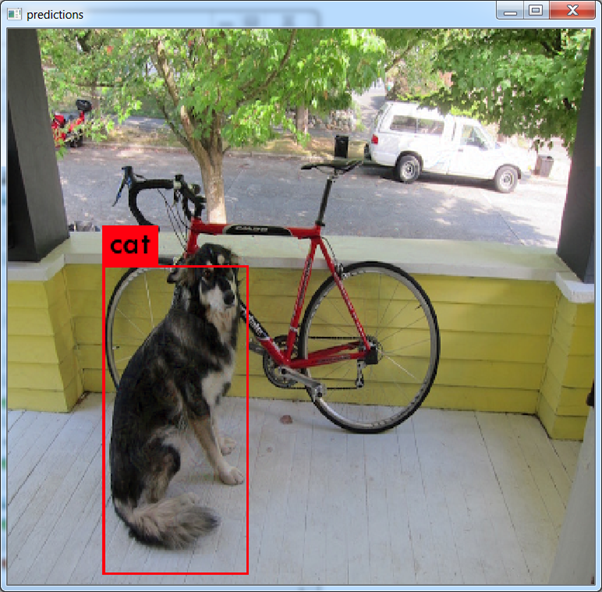
For example, the network can modify a training image that contains a dog, such that the network classifies it as a cat. When the network trains on this modified image, it is forced to pay more attention to other features. (image source)

YOLOv4 Training

With the completion of our new dataset, we were able to start training more object detection models. The dataset is split using the same arrangement as used by MIT previously, which allows us to better compare the overall performance.

• 5980 images for training
• 1185 images for validation

The validation set of 1185 images are images which the detector has not seen before, and we use these to validate and benchmark the detector’s performance. All the training runs are initialised with pre-trained ImageNet weights.

Benchmark Metrics

Before we dive into the actual benchmarks and performance figures, I would like to go over the metrics used to evaluate object detection algorithms. This includes IOU, precision, recall, AP, mAP.

• IOU is the intersection over union, and this measures how well the detected bounding box measures against the ground truth label.

IOU=Area of OverlapArea of Union

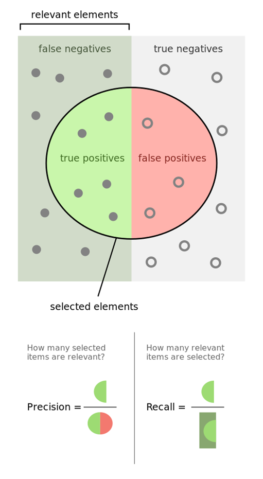
• precision and recall is illustrated as follows (image source)

• AP (Average Precision) computes the average precision value for recall value from 0 to 1.
• mAP (mean Average Precision) computes the mean AP that is averaged across all classes.

In the benchmark below, you will see mAP@0.5 and this just means that the IOU has to be greater than or equal to 0.5 for it to be considered as a positive sample.

Benchmark and Performance AnalysisPermalink

The table below illustrates the various networks which have been trained on our improved dataset, except for the YOLOv3 MIT, which is included as a point of reference. However, the model and dataset difference should be noted, since MIT custom network does not make use of class labels, whereas our networks perform object detection and classification in the same network. See MIT perception paper for more details.

All benchmark results make use of YOLOv3 and YOLOv4 at input 416x416 resolution.

The main improvement shown in the YOLOv3 MIT network is the inclusion of a custom data loader which improve bounding box size distribution and resolution so that they match the real-life data distribution, which minimises the domain shift between training data and real-life application data. This brings a significant improvement over the original YOLOv3 network.

The default YOLOv4 network achieves very similar mAP as the MIT YOLOv3 network. Interestingly, switching the YOLOv4 network to use the Adam optimiser and Self-Adversarial Training does not bring in much improvement. For the Self-Adversarial Training case, it is hypothesised that our model and dataset combination does not benefit much from the SAT routine since traffic cones are ‘relatively simple’ objects and there is little hidden cues or features the detectors can try to pick up, as opposed to cats and dogs or other more complex objects.

On the other hand, using custom anchors does bring some minor improvements to the detector. YOLO detection network makes predictions by predicting offsets from pre-computed anchor boxes. The anchor boxes are essentially a set of most common bounding box dimensions, and the closer they are to the actual object dimensions (in image pixel coordinates), the easier it is for the network to predict. See here for more information.

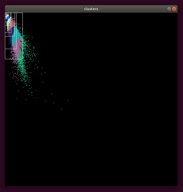
In the image above, we can see that in the black 416 x 416 image, distribution of the traffic cone sizes, and also the visualisation after k-means clustering has been performed on the training set to extract the new anchor boxes. Compared to usual everyday life objects like people, cars and aircrafts, we would expect the traffic cones to have smaller anchor boxes in general, and smaller width compared to height as most of the cones were upright when they were captured, which is exactly what is shown above. Using our custom anchor boxes, we obtain a modest gain of +0.2 mAP.

The most significant performance gain comes from the YOLOv4 Small-Object network which has a few modifications recommended by the author.

1. First, before the first YOLO detection layer, the upsample layer’s stride was increased from 2 to 4, which means that one pixel in the input will write to a 4x4 area output.
2. Second, the upsampled output is concatenated with an earlier feature map which contains higher-level details.
3. Finally, the convolutional layer after the first YOLO layer had its stride increased from 2 to 4 to “reverse” the effect the stride increase.

The result is that, before any modification, the first YOLO detection layer receives input of 76x76x24, and after the modification, it receives a feature map of 152x152x24. This means the network has a lot more information to work with to pick out the smaller traffic cones present in the image. Training a network with this modification results in a gain of +4.9 mAP, which by far outperforms the YOLOv3 MIT network.

Recall Precision Trade-off

Presented in this section are the recall-precision curves for YOLOv3 vanilla, YOLOv4 vanilla and YOLOv4 Small-Object and also the inherent trade-off between recall and precision when choosing an operating point.

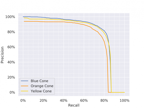
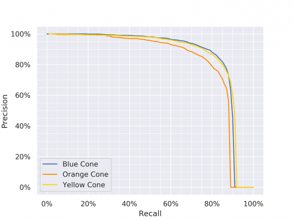
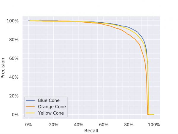
Precision Recall Curves for YOLOv3, YOLOv4 and YOLOv4 Small-Object (Click on any one of them to enter the gallery view. Then use left and right arrow keys to switch between each model.)

To minimise the number of false positives, we would like to have high precision, while maintaining a reasonable recall. For YOLOv4 Small-Object, at 90% precision, we have 75%, 80%, 85% recall for orange, yellow and blue cones respectively.

Inference Optimisation

At the point, you might be wondering whether the aforementioned networks can be deployed in real-time settings. Fortunately, the answer is yes, thanks to the optimisations that can be achieved through INT8 low-precision inference. In particular, this is achieved through the tkDNN deep neural network library that aims to maximise inference performance.

(Note that table below is sourced from the tkDNN github repository)

With batch=1, that is, 1 image input at a time, Nvidia Jetson Xavier can run up to 50-51 frames per second. This is not only limited to Nvidia’s recent embedded platforms but also any laptop/desktop equipped with relatively recent Nvidia graphics cards. Libraries like this lower the entry barrier for working on object detection projects and allows more people to jump in, test and experience accurate real-time object detection without needed extremely expensive graphics cards with large video memory.

The main trade-off is the longer than usual setup process to get all the dependencies in place.

Inference Results

The videos below show the YOLOv4 Vanilla detector running on footage captured from previous FSG competition event. The first video shows the detector running in FP32 (floating point 32) inference mode. The second video shows the detector running in INT8 inference mode, after being calibrated on 1000 images.

https://www.youtube.com/watch?v=eR-7J-I1xQQ

https://www.youtube.com/watch?v=m2LGs8waPas

Special Thanks to Nvidia

I would like to take this opportunity to thank Nvidia APAC for their generous support. The provided graphics card and Jetson AGX Xavier have allowed us to train, develop and test our neural networks. With the extremely limited budget we have for 2020, it would have been impossible to procure these devices ourselves.

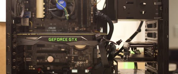
Nvidia GPU used for Training

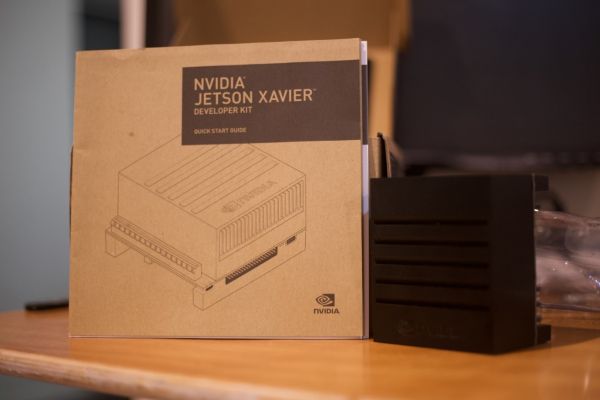
Nvidia Jetson Xavier for Testing

About the Author:

Steven Lee
Spatial & Perception Engineer, 2020