MUR Blog - Real-Time Cone Detection with LiDAR

In this article, the approach taken to detect traffic cones with LiDAR will be explored and discussed. This includes the steps taken to produce the current prototype, initial performance impression and our next steps for development.

LiDAR Pipeline and Overview

As previously mentioned in the previous blog post, the proposed LiDAR pipeline consists of the following steps. Note that the point cloud un-distortion step has been left out and will be added and discussed in a future post.

1. Obtain raw LiDAR data
2. Field of view trimming
3. Segmentation to separate ground plane and potential obstacles
4. Cluster potential obstacles
   • Cylindrical volume reconstruction
   • Filter clusters based on an expected number of points
5. Return confirmed cone position

In the last few weeks, a basic prototype of the above pipeline has been developed using ROS (Robotics Operating Systems), RViz (Visualiser used alongside ROS), PCL (Point Cloud Library) and other open-source projects. The gallery below shows the outputs captured at each step of the pipeline.

LiDAR Pipeline Visualised in RViz

Experimental Setup

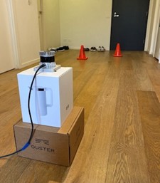Due to the COVID-19 quarantine situation, the LiDAR experimental setup was conducted in a small apartment space with as much space cleared out as possible to emulate an “outdoor” environment. The Ouster OS1-64 LiDAR was temporarily mounted in the figure image shown so that LiDAR data can be captured with rosbag, which can then be conveniently played back at any moment’s notice without setting the LiDAR.

One particular limitation of this setup is the lack of open space and an extremely limited number of traffic cones available. More traffic cones and a larger track environment would be required to better assess the performance of the implementation.

Step 1: Obtaining Raw LiDAR Data

Thanks to the open source sample codes provided by the Ouster, it was relatively straight forward to get the LiDAR up and running with ROS. However, some network changes were still required to get the wired connection working with the Ouster LiDAR. More details are available on our GitHub repository wiki page.

Step 2: Field of View Trimming

To simulate an outdoor track environment, a box filter is applied to the point cloud captured in the scene. This results in the cropped point cloud shown above.

Step 3: Segmentation

After pre-processing, the cropped point cloud is then passed to the segmentation node, which separates the ground plane from the potential obstacles which we would like to detect.

Initially, a RANSAC based plane fitting algorithm was used. However, algorithm run-time was longer than expected, which does not meet our real-time object detection requirement.

The next method chosen for segmentation is described in the paper Fast segmentation of 3D point clouds for ground vehicles. Instead of treating the point cloud as a whole, this method divides up the overall point cloud into equal segments. Each segment is then divided up into a number of bins.

Dividing the point cloud up into segments allows the problem to be tackled by 2 sub-problems of lower complexity. First is a local ground plane estimation, and the second is labeling the connected component in 2D.

Within a single segment, the lowest points of all bins are used to fit a line through them. Then all points within a specified distance to the line can then be labeled as a ground point.

There are numerous tuning parameters required for this algorithm to perform well. These will be discussed in a future blog post.

Step 4: Euclidean Clustering

A Kd-Tree based euclidean cluster approach is applied to group up all the non-ground planes. The resulting clusters are affected by the following parameters.

• Cluster tolerance
• Minimum number of points in a cluster
• Maximum number of points in a cluster

The cluster tolerance setting determines how far apart the points can be in order to be considered within the same cluster. If the cluster tolerance is too small, you may end up with too many objects. If the cluster tolerance is too large, you may end up with too few objects.

4.1 Cylindrical Volume Reconstruction

After the clustering step is completed, a cylindrical volume reconstruction step is applied. During the ground segmentation step, some points belonging to traffic cones could have been labeled as ground and removed as a result. Therefore all the points within a specified cylindrical volume are recovered and added back into each individual cluster to ensure that we have as many points as possible before we apply the filter for our next step. More details is available in a previous blog post.

4.2 Expected Number of Points

Now, a rule-based filter can be applied. Since we know the exact dimensions of the traffic cones we are working with, we can exploit this prior information and calculate the number of expected points in a cluster.

The parameters used to determine points are:

• D distance to the cluster which is 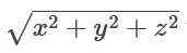where (x,y,z) is the position of the centroid of the cone

• r_v vertical resolution of the LiDAR
• r_h horizontal resolution of the LiDAR
• w_c width of the cone
• h_c height of the cone

4.2.1 Derivation

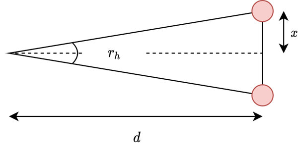
Consider the diagram above, the two red points are adjacent points in a horizontal point cloud slice. From this, we can derive the following.

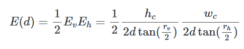
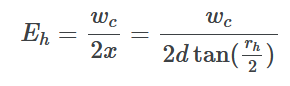
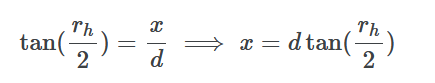Then we can find the number of expected points for the horizontal case. w_c is the width of the cone, and we expect 1 point for each 2x interval. This can then be used to determine the total number of expected points in a horizontal plane given the width of the object.

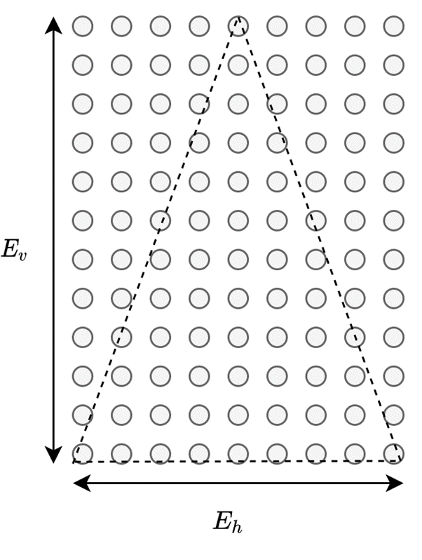
The expression for E_v, the expected number of points in a vertical scan, can be derived in the same way, except that we use r_v and h_c in the vertical case.

In the image below, a hypothetical frontal view of a rectangular point cloud is provided. Consider every circle as a point in the point cloud, we can compute the total number of points by finding the product Ev⋅Eh. However, a cone-like object has a triangular frontal cross-section as illustrated in the dashed lines below. Therefore, a factor of 0.5 is applied, giving us the expression for computing an expected number of points based on distance.

The expected number of points can then be used as a rule-based filter to eliminate non-cone-object clusters.

Step 5: Mark and Return Cone Positions

After the filter has been applied, (hopefully) we are left with only positive cone clusters. We can then take its centroid position and use that to mark its position visually in RViz and/or pass that onto the SLAM node.

Results

The video below demonstrates the traffic cone tracking capability of the prototype implementation. Note that this is not representative of how well it would scale to 40 or 50 cones on a larger race track. It is recommended to set the quality of the video to 720p for the best viewing experience.

Discussion

Qualitatively, the algorithm works well and is able to track the cones closely and robustly. However, occasionally the detection markers would pop in and out, indicating that the filtering step is not as well-tuned as it can be, causing certain cones to be missed.

In addition, there are edge cases where this implementation breaks down, namely when the cones are positioned in front and behind each other. This is reasonable as the LiDAR sensor cannot detect objects hidden/occluded behind another object.

Interestingly, the algorithm handles the side-by-side adjacent cone case relatively well in this small test area. However, further tuning would be required for the segmentation and euclidean clustering steps to ensure robust performance in much larger areas.

Next Steps

• Proper performance measure of various nodes in the pipeline
• Quantitative measure of cone detection performance
• Develop a simulation for better testing (in quarantine scenario)
• Test algorithm with a larger test area and add up to 40 cones

About the Author:

Steven Lee
Spatial & Perception Engineer, 2020